The story of BERT-ian era

There are many NLP tasks like text summarization, question-answering, sentence prediction to name a few. One method to get these tasks done is using a pre-trained model. Instead of training a model from scratch for NLP tasks using millions of annotated texts each time, a general language representation is created by training a model on a huge amount of data. This is called a pre-trained model. This pre-trained model is then fine-tuned for each NLP tasks according to need. 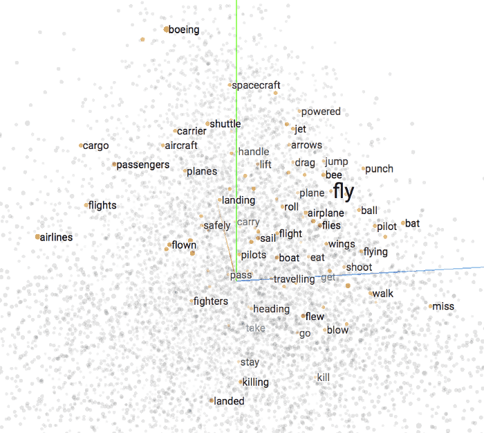Let’s just peek into the pre-BERT world… For creating models, we need words to be represented in a form understood by the training network, ie, numbers. Thus many algorithms were used to convert words into vectors or more precisely, word embeddings. One of the earliest algorithms used for this purpose is word2vec. However, the drawback of word2vec models was that they were context-free. One problem caused by this is that they cannot accommodate polysemy. For example, the word ‘letter’ has a different meaning according to the context. It can mean ‘single element of alphabet’ or ‘document addressed to another person’. But in word2vec both the letter returns same embeddings.

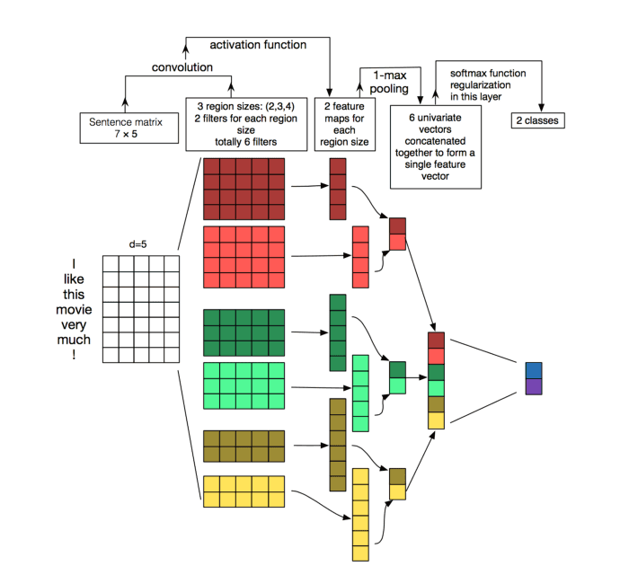
To overcome this, context-based models were created. One such is created using CNN. They follow the same approach to NLP as they have done for image processing. In Image processing, the nearby pixels have a relation and CNNs are used to understand this correlation between nearby pixels. In the case of texts, CNNs uses a matrix where the rows represent words and the number of columns depends upon the embedding size you need. If it is an n*m matrix, then “n” columns represent “n” words that we have given as the input and “m” denotes the dimension of the embeddings. Then filters are used to convolve to extract features which are in turn soft-maxed. Even though this method is quite fast considering RNNs for the same context-based approach, the relationship between tokens/words in a sentence are not similar to pixels which can be understood by their positioning. Contextual meaning has more to do with their positions.

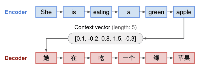
Then we have sequential models created using RNNs. It processes the words sequentially one by one either from right to left or left to right. In the case of machine translation, these consists of an encoder and a decoder (both RNNs). The encoder has 2 inputs, the word and the contextual vector. Contextual vector captures the contextual relationship of a word. The number of contextual vectors generated depends on the hidden states used in the encoder. When sequentially inputting each word(which is first converted to embeddings using a suitable algorithm), each time it outputs a context vector which is backpropagated as the input along with next word. Finally, after the whole sentence is processed, the final context vector is passed to the decoder. The decoder uses this input to generate the sentence in the target language, outputting words one by one. The problem with this approach is, RNN cannot retain long-term dependencies due to vanishing gradient problem.

As an improvement, LSTM (Long Short Term Memory) was introduced, which is an RNN with internal memory. Now RNN can, therefore, remember contexts for a longer period, providing them with a better understanding of the text they are given. But LSTM too has shortcomings similar to vanilla RNN which is evident after 2 or more layers. So now the bad guy in the current scene is ‘long-term dependencies’ which cannot be fulfilled due to vanishing gradient problem. Attention everyone, attention models are here to save the day.

As an up-gradation to the seq2seq model, an attention mechanism is used between the encoder and decoder (for machine translation). Earlier only context vector from the last hidden state is passed to the decoder to produce the translation in the target language. But if the input text is too long, the single context vector cannot retain the import segments. So using attention mechanism is like highlighting the important words in the input, which is then passed to the decoder for translation. Another use of attention mechanism is learning the alignment between the input and output. For example, we want to translate the English sentence, “What is the weather like?” to French which is “Quel temps fait-il”.

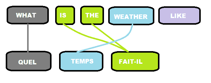
Here the positional correspondence of input and output is as above. There is no guarantee that words in the same positional index are more related. This is exactly what alignment scores do. So in short alignment scores help us in matching the input segment with corresponding output segment. The input to this attention mechanism is the context vectors generated in the hidden states of encoders. If all the hidden state output is passed to Attention, then it is called Global attention and if a subset of it is passed then it is called Local attention. The calculation for simple attention score is as below: At first, pass the final encoder hidden state value to the decoder to produce an initial decoder hidden state value(DHS1).

1. Dot product each of the hidden state(encoder) vector with DHS1.
2. Suppose if the encoder hidden state has a dimension of 3 and we have 2 encoders hidden state. Now after step 1, we have 2 vectors with dimension add each element of the vector together to produce a scalar. And finally, we have 2 scalars.
3. To normalize the above-derived number softmax the score.
4. Multiply each of the encoder hidden state vectors with the softmax-ed score. This is the alignment vector.
5. Add all the alignment vector together to produce the context vector.

This context vector is passed along with the previous output of the decoder (concatenated or added) to the decoder.

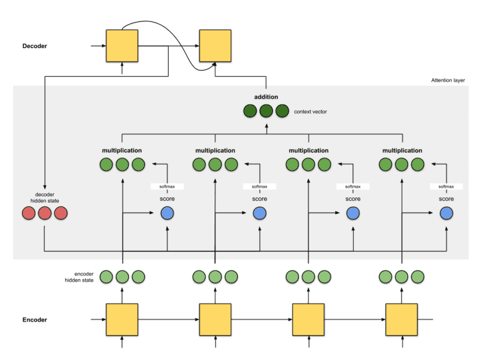
Now that is attention model. But things don’t end there. There is more. The self-attention. It is the mechanism through which the relationship between different words in the input sentence is derived. For instance, if the input sentence is, “I loved the short skirt, but the long dress looked better on me. So I was confused about buying it.” What does the word “it” refers to? We can only identify after reading the whole sentence. To understand if “it” refers to the skirt or dress, we need self-attention. Self-attention is mainly used in machine reading algorithm, where it tries to understand the text given to it. In this method, there is a word embedding matrix which is multiplied by 3 other weight matrixes to produce key, value and query matrix. Key and Query matrix have the same dimension whereas value matrix has the dimension as that of the output. The (key, value) pair represents an embedding while a query is the compressed form of the previous output. A score is calculated for each word such that it amplifies words that are important to the context and drowns that aren’t important. Let’s look at this example to understand the scoring mechanism. “The dog is running.” To find the attention vector of “running”:

Score3(“running”)
 = Query(Embedding("running")). key(Embedding("is"))
Score2(“running”)
 = Query(Embedding("running")). key(Embedding("dog"))
Score1(“running”)
 = Query(Embedding("running")). key(Embedding("the"))

Instead of dot-product, any other function can also be used. Softmax each of the scores, which gives the alignment score.

softmax(score1,score2,score3)= [0.1, 0.5, 0.2, 0.0]
[The last zero value is the score of "running" calculated against itself]

The context vector is calculated by multiplying each of the above scores with its embedding value and finally summing it up.

context vector =
(0.1*value(embedding("the")) + 0.5*value(embedding("dog")) + 0.2*value(embedding("is")) + 0.0*value(embedding("running")))

This multi-headed attention-mechanism is used in creating the transformer model. Multi-headed means it uses 8 different key, value and query matrix for each encoder, thus creating different subspaces. The transformer model consists of 6 encoders and decoders stacked up.

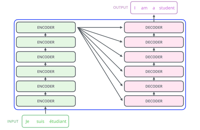
Each of the encoders consists of multi-head attention and a feed-forward network. While each of the decoders consists of a self-attention layer, attention layer (as found in seq2seq) and a feed-forward network. Read more about the transformer structure here.

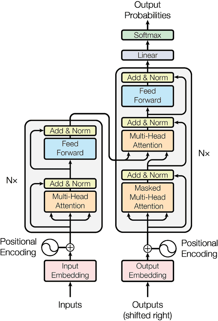
BERT stands for Bidirectional Encoder Representation of Transformers. It’s made up by stacking up the encoder portion of a transformer. Encoders are by default bidirectional, or in more accurate terms directionless as they take the whole input sequence in one go to understand the context and encode the words. The output of BERT is a representation for each input word. Before processing the input, these sequences are mapped to 3 other embeddings, i) [CLS] tokens are added at the beginning of every input.[SEP] tokens are added at the end sentences to separate them. ii) positional embeddings: indicated the position of input tokens. iii)segment embeddings: each sentence has different of these embeddings. These suggest which tokens belong to which sentence. Thus these 3 embeddings are mapped to the input which is fed into the encoders.

There are 4 versions of BERT available:

1. BERT base: It contains 12 layers with 12 attention heads
2. BERT Large: It contains 12 layers with 16 attention heads
3. BERT Cased and Uncased: depends on whether they are case sensitive

When it comes to the training of BERT model, it uses a very different technique than other models. Because as encoders can see the target through the layers, the training becomes trivial. Therefore BERT is trained with 2 novel techniques: 1) Masked Language Modelling 2)Next sentence prediction. These are 2 unsupervised predictive tasks which do supervised learning. Masked Language Modelling: In this technique, 15% of input tokens are replaced with [MASK] token. Then the encoder of BERT is made to predict the masked words. Next sentence prediction: Model takes 2 sentences and predict if the second sentence comes after the other. This technique is important as we need the model to learn sentence correlations. While training, half of the data contains the sample in which the second sentence is the next, while the rest of the sample contains a random second sentence. The encoder can identify different sentences from the [SEP] token inserted during the input to separate sentences. These tasks together train the encoder stacks to produce BERT. To fine-tune BERT for different tasks, we can add different layers, like a classification layer to produce state-of-art results for the task. These are similar to transfer learning in which we use a pre-trained model and add layers on top of it. Yeah! That’s it. And that’s all BERT is in short!