Generative models vs Discriminative models

GAN (Generative Adversarial Network) are, as the name says, Generative models.

So let’s break it down. What are generative models? Broadly speaking we have two kinds of models: Generative and Discriminative. The models that we built for classification tasks are discriminative like SVM, logistic regression. These models try to build a functional relationship between the training samples and their labels, i.e., a mapping from X (samples) ⇒ Y (labels).

While Generative models like those based on Naive Bayes or Hidden Markov models have a different approach. They first learn the distribution of data of the dataset (X). Thus, they will generate new samples for the dataset based on the distribution they have learned from the dataset. Thus the approach of Generative models is the opposite of that of Discriminative models. They try to predict X from the given Y (label).

The basic structure of VAE

So why are these GANs so cool? To understand their brilliance, let’s try to understand another predecessor of GAN, the Variational Autoencoder (VAE).

VAEs have 2 parts or networks, 1) Encoder & 2) Decoder network (oh yeah! We all know that). To give a birds-eye view of what it does, if you give an image (let’s call that input image X) to the encoder network.

After X passes through the encoder, the encoder produces certain values, which are are the features of the images learnt by the encoder model. These values or features outputted by the encoder are called latent variables.

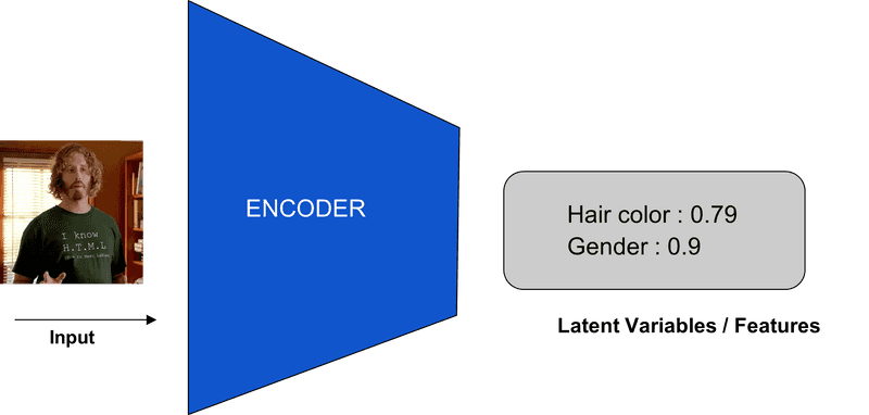
This process can be considered similar to compressing an input. These latent variables when fed to a decoder network will reconstruct the image, X.

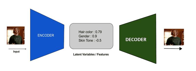
From the basic model structure shown above, it can be inferred that there are 2 networks, encoder and decoder, and these two learns 2 different sets of weights, and , respectively.

Let’s call the latent variables, z. As both are generative networks, they will learn the probability distribution similar to the input dataset’s data distribution.

The encoder will learn the probability distribution ie, predicts z given an input x for the distribution q defined in . Similarly, the decoder learns the distribution , ie, reconstructs the image x given latent variables z in the probability distribution p in . Thus both the networks are trained to learn and .

What makes VAE special is the extra stochastic layer before giving the latent variables. This is done by predicting probabilistic parameters, mean and standard deviation value for each of the features, thus instead predicting a single value for each feature (z), a latent space described by mean and standard deviation is obtained. In simple terms, z can be randomly sampled from the distribution whose mean is and the standard deviation is .

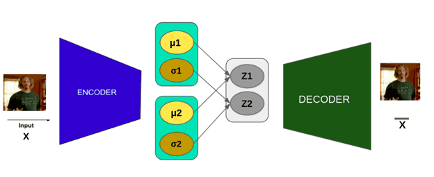
The difference between the reconstructed image () and the input image (x) gives the loss which is called reconstruction loss.

Reconstruction loss:

To reduce the overfitting of z in latent space as well as to ensure the continuity and completeness of latent space (z) in every point the Loss function for the encoder has another term added to it, other than the reconstruction loss,

Loss = Rectruction loss + Regularization term(D)

KL divergence is used for regularization as it can compare the closeness of two distributions. Also, a hypothesis or prior (P(z)) is introduced into the regularization term to place some constraints on the distribution. A Gaussian distribution is usually used as the prior or hypothesis.

Regularisation term:

Another issue with this model is that it is non-trainable because there is a stochastic layer due to the probabilistic nature of the model. The value of z is randomly sampled out from the latent space determined by and .Therefore no gradient can be obtained for this layer, thus impossible to do the backpropagation. One beautiful approach to solve this is the reparameterization technique.

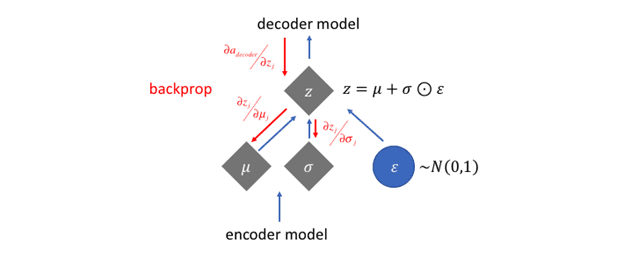
Here the stochastic nature of the z node is changed to another node, which samples from Gaussian distribution to give a value . Then shifts this value by and scale it by . This ensures that the random nature is still preserved while during the training phase this node is avoided which enables back-propagation.

There is one more detail to care of before finalizing the loss function equation. The encoder model outputs some latent variables which stand for each feature of the image. By changing the value of one of the latent variables, we must be able to change that feature of the input image, say, hair colour, without affecting other feature values like skin tone which is known as the perturbation. To enable this the latent variables should be independent of each other or De-entangled. For the de-entanglement, another variable is introduced in the loss function, .

Loss function = reconstruction loss + regularisation

Now let’s dive into GANs GANs are another generative models like VAEs which are trained in an unsupervised approach. So what’s the key difference between the two. What VAEs does is simple as encoding a data space and decoding that. So the input for the decoder is provided by the encoder which in turn is fed with one of the inputs of the data space which is converted to latent space vectors. Therefore a high dimensional input is turned into low dimensional in the encoder.

But in GANs the scenario is a little different. GANs can produce generate data that closely resembles data space. If the dataset contains different images of a human face, GANs trained on this data will be able to produce a “new” face that is not part of the dataset. So this explains the term “Generative” in Generative Adversarial Network. In contrast to VAEs, GANs produce this from low dimensional data. This low dimensional data is converted to high dimensional data ie, the output image. The low dimensional data that is fed can be any random value or noise. GANs are trained in such a way that they fit this noise into the distribution of the original dataset and produce new data points in the distribution.

In the training phase, GANs consist of two models. One is the Generator that produces the image (or any other type of data) that resembles the original dataset. Then we have another model, which tries to predict the input given to it is from the original dataset or not. So it has to predict all the inputs from the generator as False as they are synthetic data and True for data from the dataset. This model is called the discriminator as it is a discriminative model used for classification. After training is done, only the generator is used for generating images.

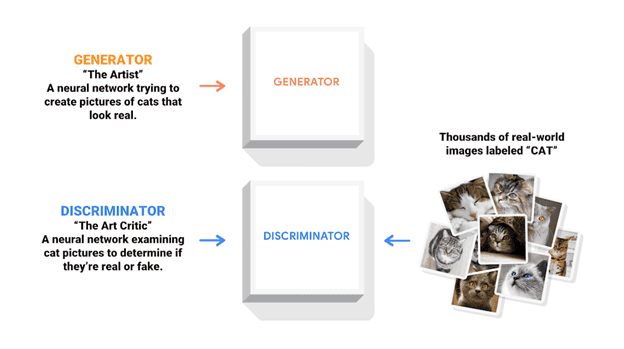
To make the working of generator and discriminator clear, let’s take the example of the Amazon fake products scenario. Let’s say Mx. Gen is someone who tries to sell fake products on Amazon. We, the customers will report it as fake as it was easily identifiable. So now Mx. Gen tries to make his product look more similar to the original brand in the outward look, thus making his product looks more like the original product. But what if the customers were smarter and able to identify a very well made fake product, then Gen will also improve his techniques to make products that looks exactly the same as the original product.

Here the customers are the discriminator model and the Mx. Gen is the Generator model. The discriminator is trained to improve its efficiency to distinguish between fake and real images. This leads to the generator producing more real-like images which are then passed to the discriminator to test its quality. The loss of the discriminator is passed to the generator to produce more accurate images.

Thus both these values are trying to fight against each other.

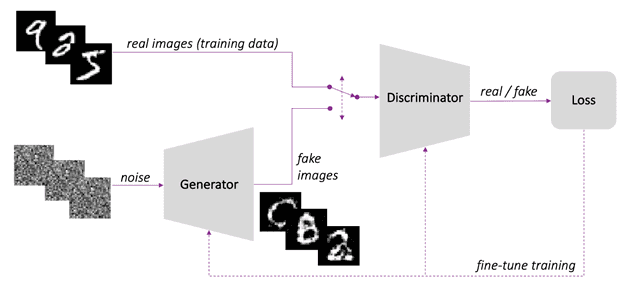
Discriminator(D) outputs the probability of whether an image is real. Thus this value ie, D(x)=1 where x is an image from the dataset. Let the noise that we give to the Generator(G) be z.

So G(z) ⇒ fake image.

By feeding this fake image to Discriminator it should output 1 ie,

D(G(z)) = 0

Loss =

We are trying to minimize log(D(G(z))) and maximize D(x) for the discriminator model.

Generally, we try to minimize a function which is our loss function. Thus we have to tweak this to a minimization problem using the Binary Cross-Entropy loss function.

BCE loss =

where x is the prediction and y is the actual label.

While training the Discriminator we need to find 2 values: 1. log(D(x)): we find this by BCE loss function, making the second term of BCE 0. To make it zero we give y=1. Thus while passing the arguments for BCE, we pass the argument as the predicted values of the discriminator and the second value as an array of 1 in the same dimension of predicted values. 2. log( 1-D(G(z)): To calculate this, we make the first term of BCE function zero by passing y=0. Hence to the loss function, we pass x as the outputs of the discriminator when generator outputs are given as its input and y, the second argument as 0. To calculate the total loss of the discriminator the average of the above 2 values is taken.

Similarly while training Generator the aim is to maximize log(D(G(z)), which is done in the same way as in the first step of the Discriminator training.

Building a simple GAN

Now let’s try to build a simple GAN from the MNIST dataset using the Pytorch library. Import the necessary libraries.

import torch
import torch.nn as nn
import torch.optim as optim
import torchvision.datasets as datasets # to download MNIST dataset
import torchvision
from torch.utils.data import DataLoader
import torchvision.transforms as transforms
from torch.utils.tensorboard import SummaryWriter

Build the Discriminator model which is a simple multilayer perceptron network. The input to this model is an image that has to be classified as real or fake. The MNIST dataset is 12828 (black and white image). Adding the dropout layer usually increases the accuracy of the model. For GANs as the activation function of hidden layers, Leaky RELU is used instead of RELU. As it is a binary classification, a sigmoid function is used as an activation function.

class Discriminator(nn.Module):
    def __init__(self,img_features):
        super().__init__()
        self.layers = nn.Sequential(
                            nn.Linear(img_features,512),
                            nn.LeakyReLU(0.1),
                            nn.Dropout(0.2),
            
                            nn.Linear(512,256),
                            nn.LeakyReLU(0.1),
                            nn.Dropout(0.2),
                        
                            nn.Linear(256,128),                            
                            nn.LeakyReLU(0.1),
                            nn.Dropout(0.2),
            
                            nn.Linear(128,1),
                            nn.Sigmoid(),
                            )
    def forward(self,x):
        return(self.layers(x))

Now, let’s build the Generator model. This too like our Discriminator is a simple multilayer perceptron. To get better results CNN can be used. The input to this model is some random noise of chosen dimension. Adding Batch normalisation has tended to decrease the training time. The output for this layer is the fake image of dimension 12828. Thus our last layer’s output size is 784 (28*28).

class Generator(nn.Module):
    def __init__(self, noise_dim, img_features):
        super().__init__()
        self.gen_layers = nn.Sequential(
            nn.Linear(noise_dim,256),
            nn.BatchNorm1d(256,0.8),
            nn.LeakyReLU(0.2),
            
            nn.Linear(256,512),
            nn.BatchNorm1d(512,0.8),
            nn.LeakyReLU(0.2),
            
            nn.Linear(512,1024),
            nn.BatchNorm1d(1024,0.8),
            nn.LeakyReLU(0.2),
            
            nn.Linear(1024,img_features),
            nn.Tanh(),
        )
    def forward(self,x):
        return self.gen_layers(x)

If you have a GPU in your system, use it for processing else choose CPU. Now let’s set all the hyperparameters. Try to play with the learning rates and see if you can come up with a better value. fixed_noise is an array that stores random numbers as noise input to the Generator to test its output.

device = torch.device("cuda") if torch.cuda.is_available() else torch.device("cpu")
lr = 0.0003
batch_size = 32
epochs = 100
noise_dim = 64
img_features = 28*28*1
fixed_noise = torch.randn((batch_size,noise_dim)).to(device)

Create the model instances from the classes.

gen = Generator(noise_dim,img_features).to(device)
disc = Discriminator(img_features).to(device)

Two transformations are currently applied to the dataset. ToTensor() converts the image to torch array and divides it by 255 thus keeping the value between 0 and 1. Then a Normalisation is applied by specifying mean and standard deviation. This value affects the quality of the images produced by the generator model, so try to explore different combinations to achieve a perfect result.

Load the dataset to a data loader.

transforms = transforms.Compose([transforms.ToTensor(),
                                 transforms.Normalize((0.5,),(0.5,))])

dataset = datasets.MNIST(download = True,
                         root ="/path/", 
                         transform=transforms)
loader = DataLoader(dataset,shuffle=True, batch_size=batch_size) 

As discussed above the loss function we will be using is BCE loss. And the optimizer is Adam.

To view the results in tensorboard, initiate a Summary Writer.

criterion = nn.BCELoss()
gen_optim = optim.Adam(gen.parameters(),lr=lr)
disc_optim = optim.Adam(disc.parameters(),lr=lr)
writer_fake = SummaryWriter(f"runs/gan_MNIST/fake lr:0.0003 batch 100")
writer_real = SummaryWriter(f"runs/gan_MNIST/real lr : 0.0003 batch 100")

Now the training begins. As we are using a sequential model, before passing the image directly to our model, we will have to flatten the inputs. The mean loss is calculated as we discussed above. Then Generator is trained in the same loop.

step =0
for epoch in range(epochs):
    for idx,(img,_) in enumerate(loader):
        batch_size = img.shape[0]
        '''not interested in predicting labels only want image'''
        img_real = img.reshape(-1,784).to(device) # 784 = 28*28*1 --> 1D instead of matrices
        outputs = disc(img_real)
        real_outputs = outputs.reshape(-1) # output shape will be (batch_size,1)
        loss_real = criterion(real_outputs,torch.ones_like(real_outputs))
        '''loss is calculated with a [1,1,1...]. This is to reduce the second term of BCE to 0.
        bce = ylog(x) - (1-y)log(1-x).
        by definition of loss of discriminator:
            max[log(D(real)) + log(1-D(G(noise)))]  BCE==> 1st term
        '''
        # calculating the second part of BCE function, making the first part zero
        noise = torch.randn(batch_size,noise_dim).to(device)
        fake_img = gen(noise)
        fake_outputs = disc(fake_img).reshape(-1)
        loss_fake = criterion(fake_outputs,torch.zeros_like(fake_outputs))
        
        loss_disc = (loss_real + loss_fake)/2
        
        disc_optim.zero_grad()
        loss_disc.backward(retain_graph=True)
        disc_optim.step()
        
        # Training generator
        '''Generator has to min{log(1-D(G(noise)))} == max(log(D(G(noise))))'''
        gen_outputs = disc(fake_img).reshape(-1)
        loss_gen = criterion(gen_outputs, torch.ones_like(gen_outputs))
        gen_optim.zero_grad()
        loss_gen.backward()
        gen_optim.step()
        
        
        
        if idx==0:
            print(f"{epoch}/{epochs}   Loss_gen:{loss_gen:.4f}  Loss_disc:{loss_disc:.4f}")
            
            with torch.no_grad():
                fake = gen(fixed_noise).reshape(-1,1,28,28)
                img_fake_grid = torchvision.utils.make_grid(fake,normalize=True)
                img_real_grid = torchvision.utils.make_grid(img,normalize=True)
                
                writer_fake.add_image(f"Fake images",img_fake_grid,global_step=step)
                writer_real.add_image(f"Real images",img_real_grid,global_step=step)
                
                step+=1

This video is the output results as seen in the tensorboard. The first row shows the fake images being produced by the generator during the training process for different hyperparameter values.

So that’s how you build a simple GAN and happy coding!